| Daron Anderson dnanderson@pcisys.net |
Tracy Petrie tracy@marcad.com |
In Project 3, we implemented Connected Components and Quasi-Connected Components "in the style of" OpenCV. Components creation also supports morphological calculation and pruning in an efficient manner. We then used these to explore background removal techniques and attempted to apply them to our original eddy-current metal fastener defect detection problem.
Connected components, when displayed, were colored using the following color palette. The colors were selected in order, starting from the first row, first column, and looping around to the beginning when more than 48 colors were required.

Intel publishes a style guide for writing OpenCV code. Where it made sense for this project, we followed them. Certain style guidelines were consciously ignored such as using spaces instead of tabs.
Most calculations were made during the construction of the connected components. Detection of edge pixels was done during the pruning pass after relabelling. The final set of morphologies identified are:
Pruning was limited to area, average value, and bounding box features. Provision was made to prune by minimum, maximum or both (for range tests). A structure, CvCCShears, and several bit constants were created to specify the pruning actions to take.
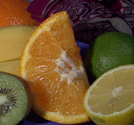
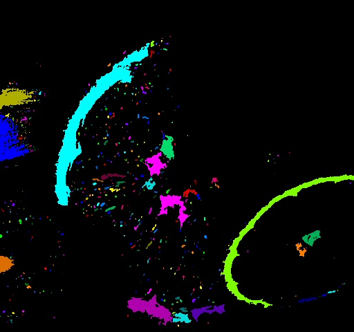
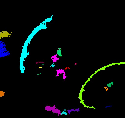
We implemented Connected Components for color and grayscale (8-bit) images using either 4-neighbor or 8-neighbor connectivity and a single threshold value (0 to 255) as the primary pixel inclusion test. Subsequent filtering was possible using the pruning structure described above. The table below shows the original fruits.jpg image and different applications of the Connected Component algorithm.
| Original fruits.jpg image |  |
| Connected Components with threshold of 150, no pruning. |  |
| Connected Components with threshold of 150, pruning with minimum area of 40 pixels. |  |
|
|
|
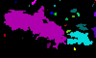
| 4-neighbor connections | 8-neighbor connections. Notice the red circles; these identify diagonal connections between components that are ignored in the 4-neighbor image to the left. |
We implemented Quasi-Connected Components (QCC) for color and grayscale (8-bit) images using either 4-neighbor or 8-neighbor connectivity and two thresholds, value (0 to 255) for both, as the primary pixel inclusion test. The high threshold allowed us to filter out componentes that may have been noise that was not filtered out by the lower threshold. A special region size was allowed to be set, to control how aggressively pixel groups were combined to form single components. Attribute calculations and morphological pruning were implemented with the same capabilities as the Connected Components implementation.
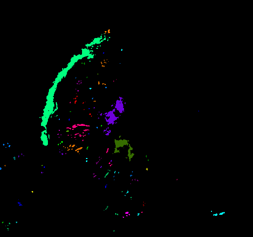
We demonstrate the effectiveness of the QCC algorithm using the same fruits.jpg image, used above. The lower threshold is set to 150, and the upper threshold is set to 180. Using simple 4-connected QCC with a region size of 4, the algorithm 'filters' out parts of the image that don't contain enough information (as determined by the upper threshold.) For instance, parts of the banana that were detected as a component using connected-components have been removed from the image.
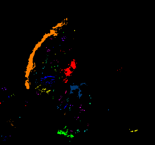
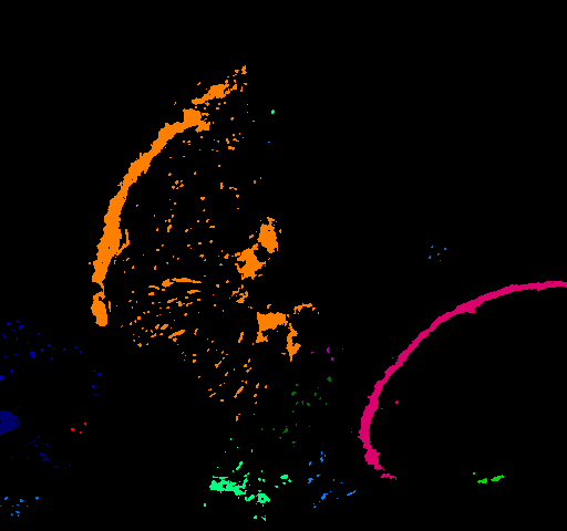
8-connected QCC was applied to the same image, with the same threshold parameters, to help group together elements that are roughly diagonal to each other,but very close together. As we progressively move toward a larger region size, the elements of each component are grouped to better reflect the actual objects in the original image. At a region size of 12, the elements of each fruit are very well grouped together. This grouping very accurately combines the elements of each fruit into the correct set of components. There are 6 detected components that correspond to 4 actual objects. This demonstrates that although we removed most of the pixels from the original image, the image still contains useful information about the physical objects, and QCC is adept at finding that information.
| QCC 4-neighbor connection. Lower threshold=150 upper threshold=180 region size=4 |
 |
| QCC 8-neighbor connection. Lower threshold=150 upper threshold=180 region size=4 |
 |
| QCC 8-neighbor connection. Lower threshold=150 upper threshold=180 region size=8 |
 |
| QCC 8-neighbor connection. Lower threshold=150 upper threshold=180 region size=12 |
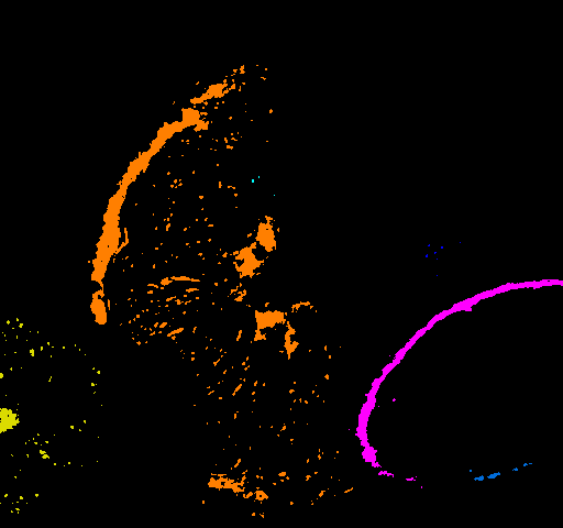 |
The following table shows the components discovered in the 8-connected image with region size of 12.
| label | area | avgValue | center(x,y) | centroid(x,y) | edgePixels | rect(x,y,width,height) |
| 1 | 6506 | 164 | (200,265) | (175,234) | 2854 | (80,59,241,412) |
| 6 | 9 | 165 | (239,169) | (233,165) | 9 | (229,160,21,18) |
| 8 | 18 | 165 | (403,235) | (395,229) | 18 | (387,220,32,31) |
| 10 | 1923 | 157 | (414,349) | (388,326) | 621 | (317,254,195,190) |
| 14 | 529 | 162 | (46,378) | (21,376) | 315 | (0,289,93,178) |
| 19 | 88 | 163 | (455,429) | (449,431) | 63 | (427,421,57,16) |
The Quasi-Connected Components algorithm has the ability to connect elements that are not directly adjacent to each other. This provides the ability to threshold out some areas of an object, and still treat the remaining areas as a single component. In this section we demonstrate this ability and compare it to the standard Connected Components algorithm. To do this comparison, we use a simple image, named 'smileyface.bmp'. Connected components sees the elements of the face as separate components, regardless of the connected-ness. Quasi-Connected Components with a large enough region size can connect the components together. The following table provides visual comparison between the algorithms and region sizes. The Connected Components algorithm always finds 4 components in this image. This may not accurately reflect the real world object that this image was taken from (perhaps this image contained a person wearing a T-shirt with the classic smiling-face icon.) As we increase the region size toward 4 (a relatively small region size), each of the components gets treated as if they are indeed part of the same overall physical object.
| Original |  |
Discovered Components | |||||||||||||||||||||||||||||||||||
| CC 4-conn |  |
|
|||||||||||||||||||||||||||||||||||
| CC 8-conn |  |
|
|||||||||||||||||||||||||||||||||||
| QCC 4-conn region size=1 |  |
|
|||||||||||||||||||||||||||||||||||
| QCC 4-conn region size=2 |  |
|
|||||||||||||||||||||||||||||||||||
| QCC 4-conn region size=3 |  |
|
|||||||||||||||||||||||||||||||||||
| QCC 4-conn region size=4 |  |
|
|||||||||||||||||||||||||||||||||||
| QCC 8-conn region size=1 |  |
|
|||||||||||||||||||||||||||||||||||
| QCC 8-conn region size=2 |  |
|
|||||||||||||||||||||||||||||||||||
| QCC 8-conn region size=3 |  |
|
|||||||||||||||||||||||||||||||||||
| QCC 8-conn region size=4 |  |
|
The Quasi-Connected Components can also utilize area-pruning. Using area pruning, the discovered components can be limited to large (or small) objects in an image. The following table shows the effect of area-pruning with different region sizes using the smileyface image. As seen in the images, the eyes of smileyface are eliminated from the resulting image unless the QCC algorihtm can connect them to another component to form a single component with area that exceeds the minimum area-threshold.
| QCC 4-conn region size=3 pruning area=12 |  |
|
|||||||||||||||||||||
| QCC 4-conn region size=4 pruning area=12 |  |
|
|||||||||||||||||||||
| QCC 8-conn region size=2 pruning area=12 |  |
|
|||||||||||||||||||||
| QCC 8-conn region size=3 pruning area=12 |  |
|
|||||||||||||||||||||
| QCC 8-conn region size=4 pruning area=12 |  |
|
QCC has the potential to be applied to many different areas. One possible application is text grouping (possibly for a preprocessor to an OCR algorithm.) Since most text that is formatted for human readability seems to tend toward grouping of words in close proximity, it is possible that QCC can be applied to find the locations of words within a document. To demonstrate this, we take an image of a basic shipping label from a major shipping company and apply QCC to it. The label is black text on a white background, so we first inverted the coloring on the label to get white text on a black background. Then we applied QCC on the label's image, with region size of 6 and lower area thresholds of 0, 225, and 1500. Using area threshold of 0, we get a fairly well grouped set of text blocks. By applying area threshold of 225, we are able to filter out some of the smaller text blocks. It is probably a reasonable assumption that text blocks that are more important to humans would be made larger, so this technique could be useful for removing unimportant text from the set of components. By applying area threshold of 1500, we removed all text blocks from the image, and leave only a barcode behind.
In the barcode scanning industry, several devices are employing a 2D imager to be able to read 1D and 2D barcodes, without the human operator having to orient the scanner. By employing QCC to the captured label image, it may be possible to implement an efficient barcode locator.
It follows that if we apply an upper threshold to the image, the barcode could be removed from the image, and only text blocks would remain, making it easy for some text-recognition algorithm to efficiently locate and decipher the possible text items from the label. (If we had more time available, we would have collected some real-world label samples from several different shipping companies and applied the algorithm to a large set of labels to determine how effective it could be.)
| Original Label Image | 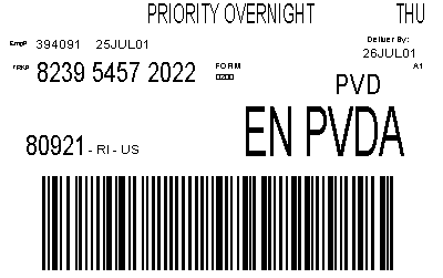 |
Discovered Components | ||||||||||||||||||||||||||||||||||||||||||||||||||||||||||||||||||||||||||||||||||||||||||||||||||||||||||||||||
| Inverted Label Image | 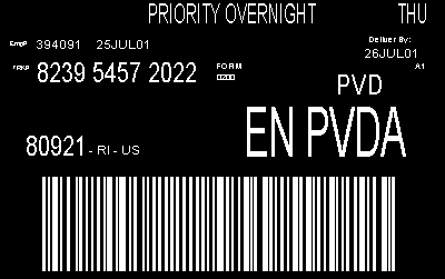 |
|||||||||||||||||||||||||||||||||||||||||||||||||||||||||||||||||||||||||||||||||||||||||||||||||||||||||||||||||
| QCC 4-conn region size=6 pruning area=0 | 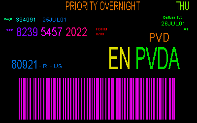 |
|
||||||||||||||||||||||||||||||||||||||||||||||||||||||||||||||||||||||||||||||||||||||||||||||||||||||||||||||||
| QCC 4-conn region size=6 pruning area=225 | 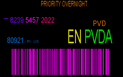 |
| ||||||||||||||||||||||||||||||||||||||||||||||||||||||||||||||||||||||||||||||||||||||||||||||||||||||||||||||||
| QCC 4-conn region size=6 pruning area=1500 | 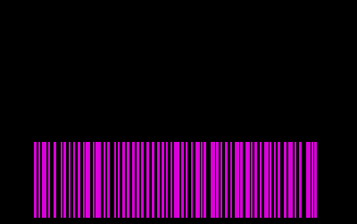 |
|
It is possible to use an eddy-current scanning device with different step sizes on each axis. Usually, an averaging technique is employed to fill in the 'gaps', as well as smooth out the image. It may be desirable to fill in the 'gaps' between each axis in the raw data set before applying an averaging algorithm to the data. This type of preprocessing would allow the initial 'filling' in to be very localized to the real data, which may provide a more accurate method of interpolation.
Using QCC, we can quickly identify the basic objects in the image. First we created an image of the raw eddy current data and treated each data point as a single pixel in the image. The image step size was kept the same for each axis, to ensure the geometry of the scanned surface was kept in tact. Then we applied QCC to the image and found the 2 components in the test image. Using the information about these two components, we could interpolate the values of the missing pixels in a very localized fashion. It may even be possible to extend the basic QCC algorithm to perform this interpolation on the fly, but we did not have enough time to experiment with this.
The following table shows the original raw data image, and two levels of lower threshold applied to the image. The different levels of threshold demonstrate two possible images that the interpolation could be applied to. (The usefulness of this pre-processing technique may be investigated in the near future, if we have time available.)
| Original Image | 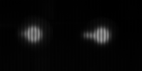 |
Discovered Components | ||||||||||||||||||
| QCC 4-conn region size=4 lower threshold=150 upper threshold=180 | 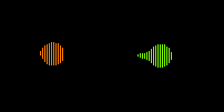 |
|
||||||||||||||||||
| QCC 4-conn region size=4 lower threshold=20 upper threshold=180 | 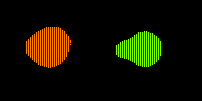 |
|
Two other avenues were explored based on the efficient derivation of CC morphologies. The first hypothesis explored the idea of using the centroid data with the center data to project the direction of a (single) defect. The idea was that the defect would have a stronger impact on the placement of the component center than on its centroid. This can best be illustrated with an imagined image of a lollypop with a one-pixel "handle." The center of a component shaped like this would be somewhere in the middle of the handle. The centroid, on the other hand, would still be somewhere in the lollypop circle itself.
| Original Image | 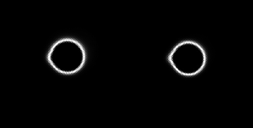 |
|||||||||||||||||||||
| Defect Detection Using CC | 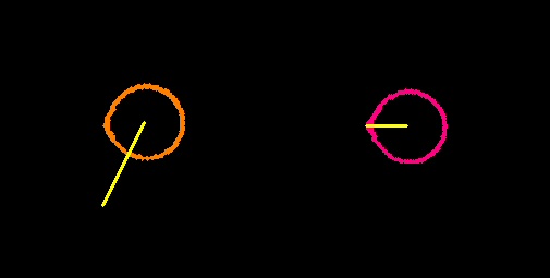 |
|||||||||||||||||||||
| Defect Detection Using Previous Method | 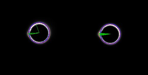 |
|||||||||||||||||||||
| Discovered Components |
|
Attempted detection on test data with small defect. The projected ray appears to work on the second rivet but clearly is off on the first rivet. Examination of the discovered components reveals that the difference between the center and the centroid is only one or two pixels. This results in calculations that are too course. With only one pixel deviation, angle choices are limited to 0, 45, 90, 135, 180, 225, and 270 degrees.
Second Example
| Original Image | 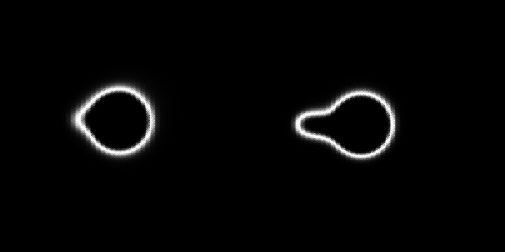 |
|||||||||||||||||||||
| Defect Detection Using CC | 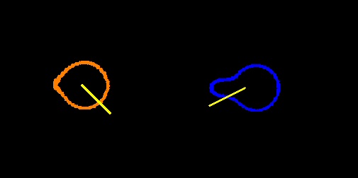 |
|||||||||||||||||||||
| Defect Detection Using Previous Method | 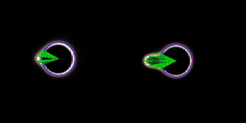 |
|||||||||||||||||||||
| Discovered Components |
|
Attempted detection on test data with a larger defect. Neither projected ray appears to work in this image. Examination of the discovered components reveals that again the difference between the center and the centroid is only one or two pixels.
Two methods of background detection were tried. The first approach used for background removal (i.e. constructing a background without objects that could subsequently be used to identify foreground objects) was to construct connected components in both the original image and subsequent images and to look for components that had appeared to move. Movement was classified as one of three types: unmoved, partial moves (object overlaps itself) and complete moves (object has no overlap or no longer exists in the scene). If an object (represented by a connected component) appeared to move completely, the entire set of pixels from the second image identified by its position in the first image could be copied back into the first image to construct the background model. If an object only partially moved, then the difference in pixels needed to be calculated to construct the mask. Objects that appeared not to move (within some threshold) were ignored and objects that no longer appeared in the second image were considered to have completely moved.
Of critical importance is the method of identifying the same object in both images. Since our connected components are constructed with simple thresholding and have minimal morphological attributes, our algorithm was simply to compare the average value and bounding box. As seen in the first test set, this was successful as long as the object being moved was solid and as long as the Hue channel of HSV color space was used. A more realistic approach might be to construct components from similar values rather than from thresholded values and to possibly incorporate some sense of texture.
| Original Positioning of Objects | 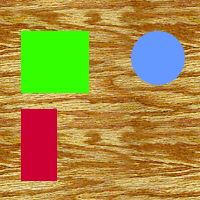 |
| The green square has partially moved, the red rectangle has completely moved, and the blue circle is unmoved. | 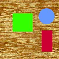 |
| Black areas represent the mask that will be applied to initial and secondary image. In the initial image, it is used to mask out the bits. In the second image, it is used to mask in the bits. | 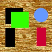 |
| Result of ORing together the two masked images. | 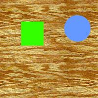 |
This test set featured one simple solidly colored object moving against a contrasting and highly textured background. We show the (successful) results using the HSV color space and the (unsuccessful) results using regular simple Grayscale color space.
HSV Color Space
| First image | 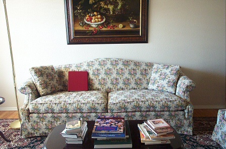 |
| Second image | 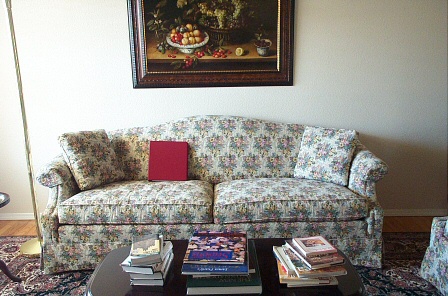 |
| Hue plane of first image in HSV space | 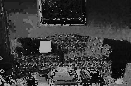 |
| Hue plane of second image in HSV space | 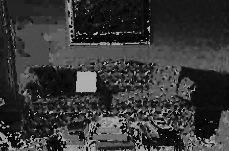 |
| Connected components of first image | 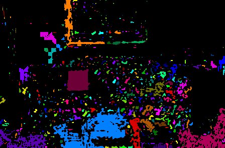 |
| Connected components of second image | 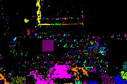 |
| Mask created by found items that appeared to move either partially or completely | 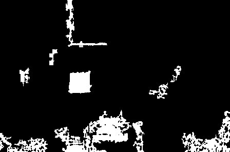 |
| Pixels extracted from second image | 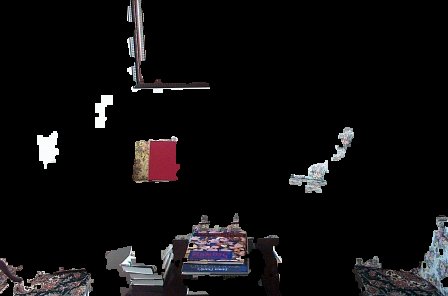 |
| Pixels removed from first image | 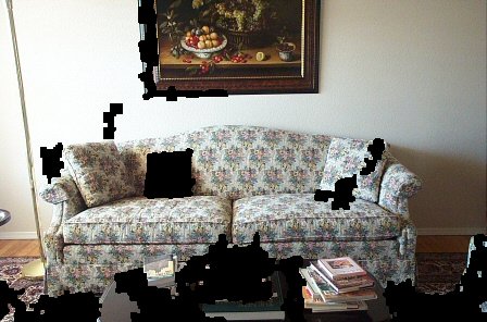 |
| Merged image (new background "model") | 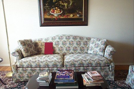 |
Subsequent applications of the process above:
 |
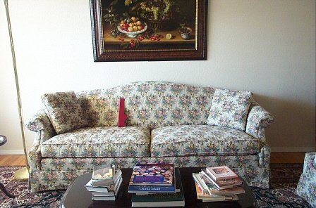 |
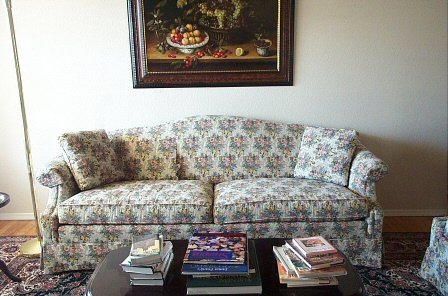 |
Grayscale Color Space
| First image, grayscale | 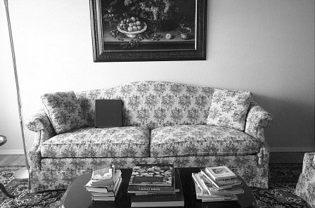 |
| Second image, grayscale | 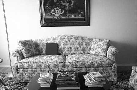 |
| First image, connected (blurring and closing applied) | 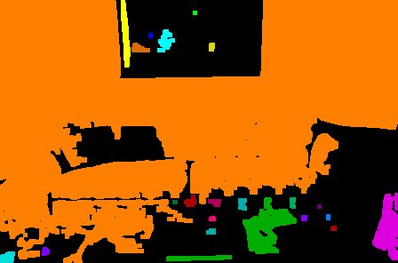 |
| Second image, connected (blurring and closing applied) | 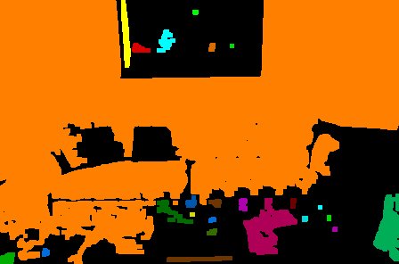 |
| Mask | 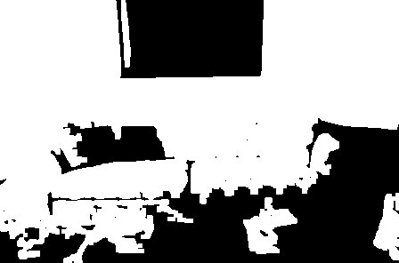 |
| Pixels extracted from second image | 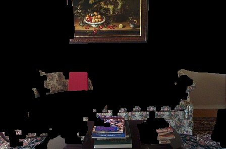 |
| Pixels removed from first image | 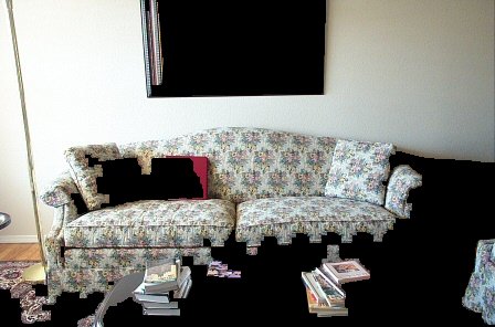 |
| Composite image. Notice the overlap of the red binder. | 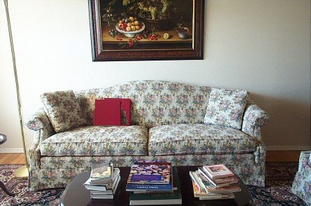 |
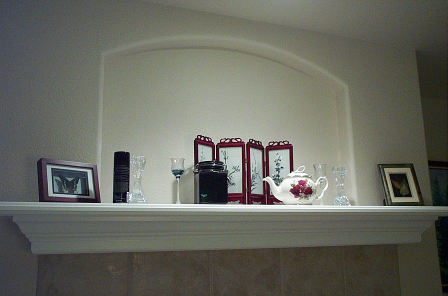
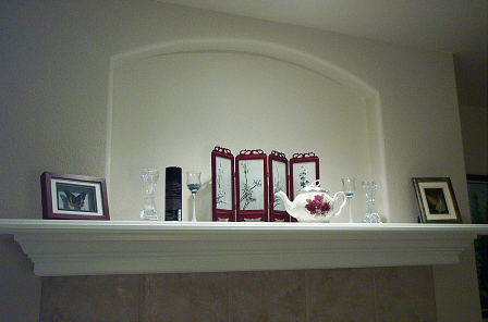
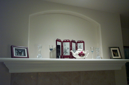
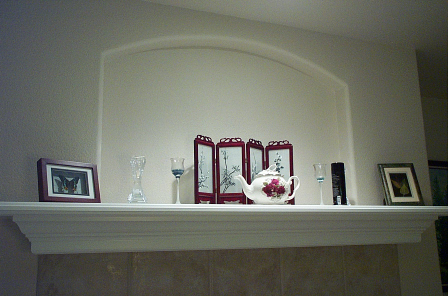
This test set featured several difficult conditions. Two of the objects are black against a very light background which is bad for simplistic thresholding. One object has a complex pattern and is moving slowly. One of the black objects eventually overlaps the second black object. We show the (successful) results using the HSV color space and the (unsuccessful) results using regular simple Grayscale color space.
Initial Image Sequence
 |
 |
 |
 |
HSV Color Space
| Hue plane of first image | 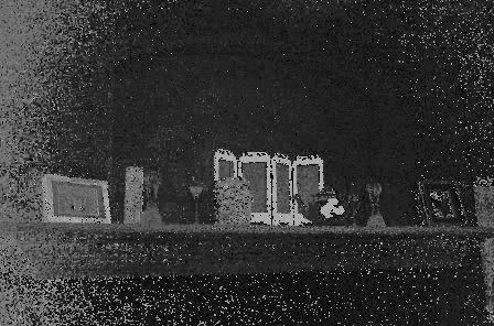 |
| Hue plane of second image | 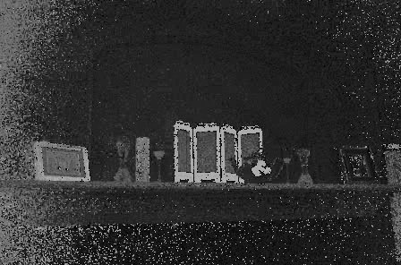 |
| First image connected components | 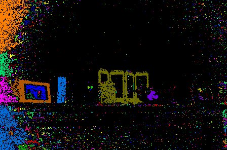 |
| Second image connected components | 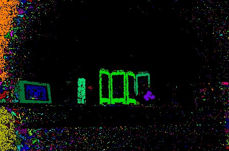 |
| Mask | 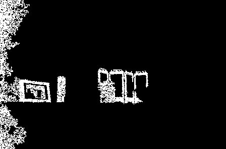 |
| First image, pixels removed | 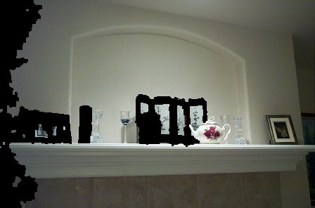 |
| Second image, pixels extracted | 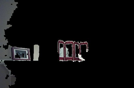 |
| Merge of first and second images. Notice the successful removal of the two black objects but the unsuccessful removal of the teapot. | 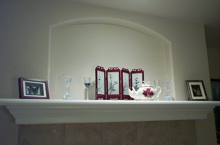 |
| Merge of first and third images. Notice the reappearance of the black area at the edge of the screen. Looking at the original images, you can see that the tall black can is overlapping the rectangular black container now and, as a result, gets masked into the image. | 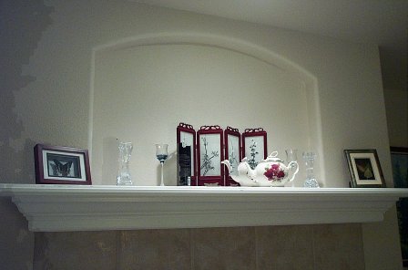 |
Grayscale Color Space
| Grayscale first image | 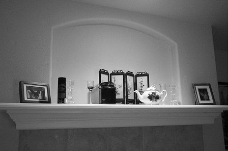 |
| Grayscale second image | 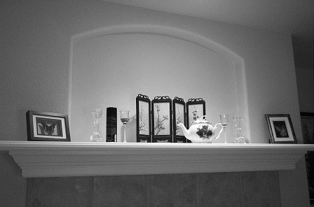 |
| Connected first image | 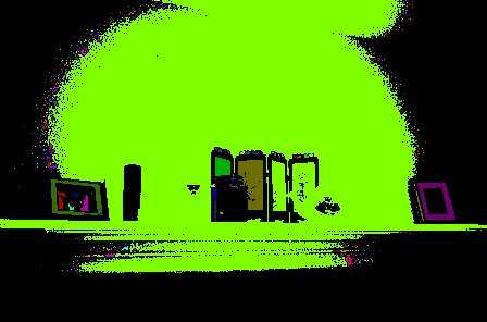 |
| Connected second image | 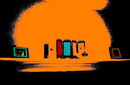 |
| Mask | 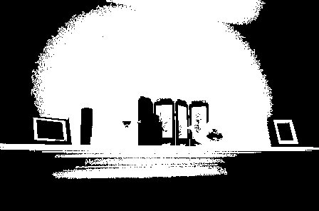 |
| Pixels extracted from second image | 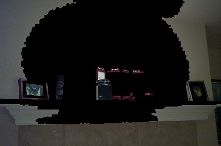 |
| Pixels removed from first image | 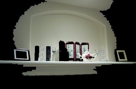 |
| Merged image. Notice that nothing has actually been successfully removed but that in fact the black canister has been dupplicated. | 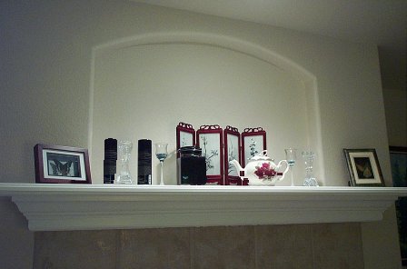 |
The second method used image differences. After taking the difference both ways (A-B, B-A) and ORing them together to get the equivalent of an absolute value difference, the difference image was connected and the list of connected components compared with the connected components of the secondary image. A challenge with this approach is finding if a connected component in the difference image exists in the second image. Our simple approach is find components in the second image that have a pixel at the center of the difference component and, if the average value is close, we make the assumption that it is a fragment of the object in the second image (and therefore does not exist in the first image).
Again, extracting the Hue plane created some level of success while a simplistic grayscale image failed. We only show the hue results which are mixed.
Test Set 1
| OR'd differences thresholded | 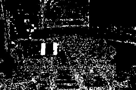 |
| Connected components of second image | 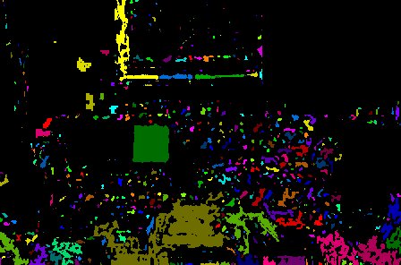 |
| Connected components of difference image | 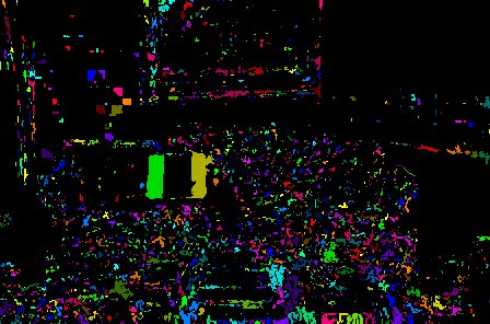 |
| Resultant mask (before morphology) | 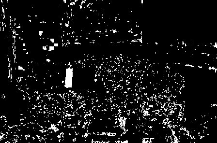 |
| Pixels eliminated from first image | 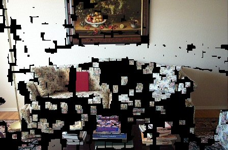 |
| Pixels included in second image | 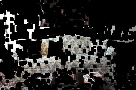 |
| Merged image (first and second) | 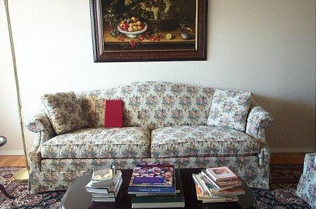 |
| Merged image (first and third) | 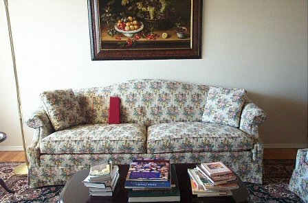 |
| Merged image (first and fourth) | 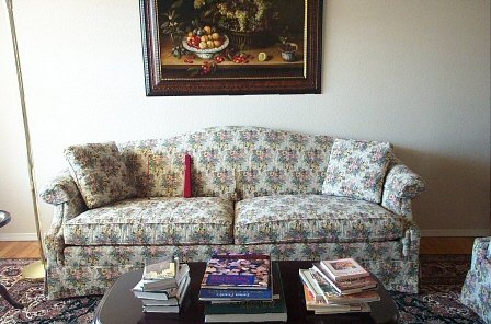 |
| Merged image (first and fifth). Notice the reappearance of the red binder now that there is no overlap. This is partially an artifact of not building a progressive background model but rather taking the first image and only constructing models from it and a single later occurring image. | 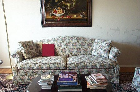 |
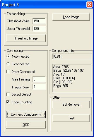
| Experiments with the functionality contained primarily in cvconnect.cpp/h
and BkgdDlg.cpp/h files were conducted using a utility that allowed us to
play with various parameters. The zip file
for the entire project is here. The cvconnect.cpp/h files are our
"in the style of OpenCV" candidates.
Component info is obtained by clicking on a component drawn on the display of the created OpenCV window. |
 |